3 Network data: how to store and use network data
3.1 Different formats to store network data
Relational data consist of nodes and edges between these nodes. Data on the nodes—nodal attributes—can be stored in the conventional way of storing observational data: in a data frame where each row corresponds to each node (observation) in the network and columns to variables (eg. gender). The edges that make up a network need to be stored in a slightly more complex manner.
Take the following network of friendship relations between members of the Swiss national soccer team, leading up to the 2014 world championship. Players were asked in a series of interviews with each player in Neue Zürcher Zeitung about their friends in the team. This information was used to create a network dataset for illustrative purposes. https://www.nzz.ch/sport/wm-2014/portraetserie-der-schweizer-nationalspieler-1.18315579
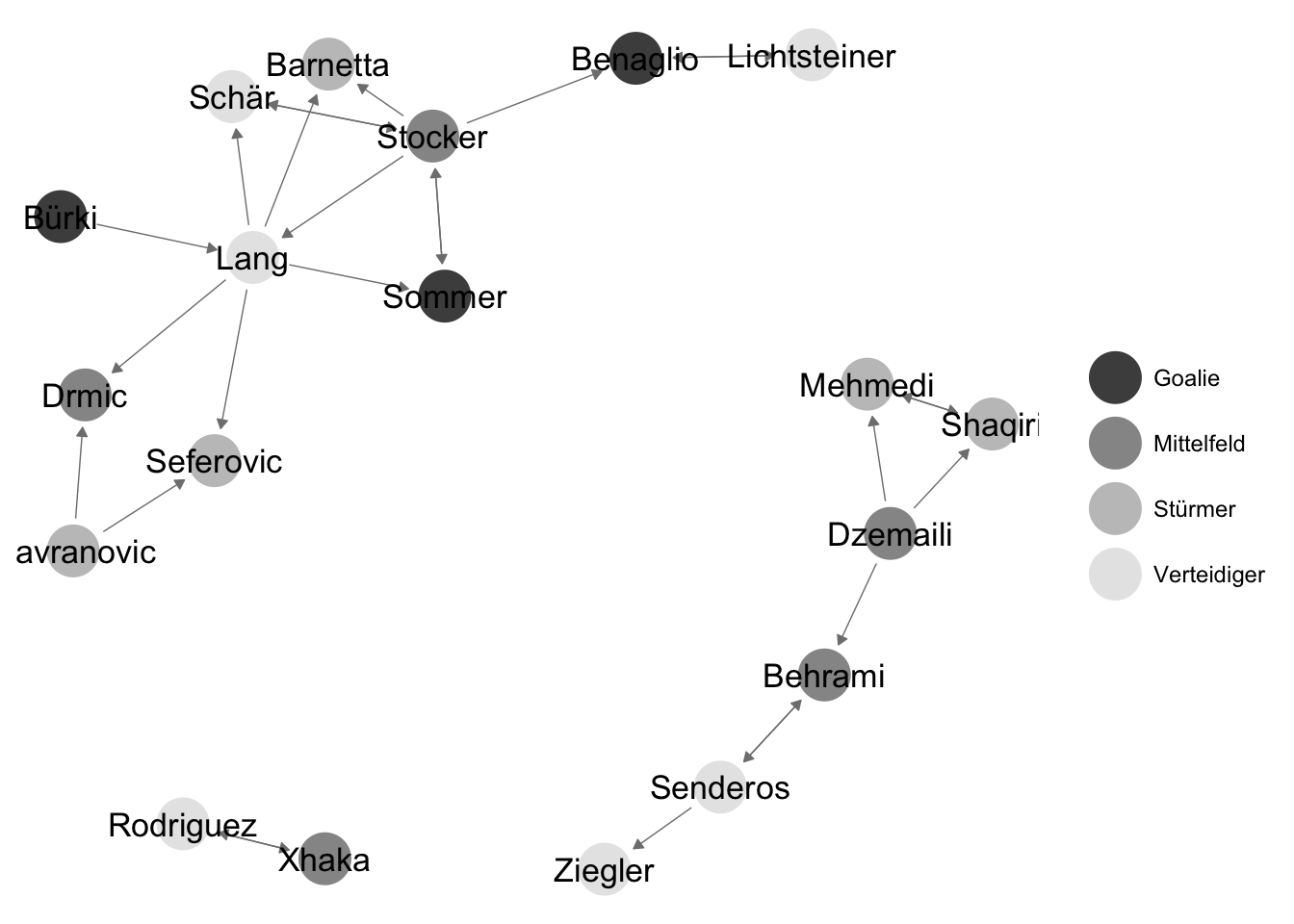
Figure 3.1: Friendship relations between members of the Swiss national soccer team
To store the network data leading to the network plot, the sender and target nodes of each edge in the network have to be recorded. There are multiple ways of storing network data. The simplest form is called a edgelist, where each row in a data set corresponds to a tie in the network:
##          Sender     Receiver
## 2    Gavranovic        Drmic
## 3    Gavranovic    Seferovic
## 4          Lang       Sommer
## 5          Lang        Schär
## 6          Lang    Seferovic
## 7          Lang     Barnetta
## 8          Lang        Drmic
## 9         Bürki         Lang
## 10        Schär      Stocker
## 11       Sommer      Stocker
## 12      Stocker     Benaglio
## 13      Stocker     Barnetta
## 14      Stocker        Schär
## 15      Stocker       Sommer
## 16      Stocker         Lang
## 17      Shaqiri      Mehmedi
## 18     Benaglio Lichtsteiner
## 20        Xhaka    Rodriguez
## 22 Lichtsteiner     Benaglio
## 23    Rodriguez        Xhaka
## 27     Dzemaili      Mehmedi
## 28     Dzemaili      Shaqiri
## 29     Dzemaili      Behrami
## 31      Mehmedi      Shaqiri
## 32     Senderos      Ziegler
## 33     Senderos      Behrami
## 34      Behrami     Senderos
Here the rows correspond to the edges in the network, the columns correspond to sender nodes myel[,1] and target nodes myel[,2].
An alternative way of storing network data is by creating an adjacency matrix with all unique nodes in the rows as well as in the columns:
##              Gavranovic Lang Bürki Schär Sommer Stocker Shaqiri Benaglio
## Gavranovic            0    0     0     0      0       0       0        0
## Lang                  0    0     0     1      1       0       0        0
## Bürki                 0    1     0     0      0       0       0        0
## Schär                 0    0     0     0      0       1       0        0
## Sommer                0    0     0     0      0       1       0        0
## Stocker               0    1     0     1      1       0       0        1
## Shaqiri               0    0     0     0      0       0       0        0
## Benaglio              0    0     0     0      0       0       0        0
## Xhaka                 0    0     0     0      0       0       0        0
## Lichtsteiner          0    0     0     0      0       0       0        1
##              Xhaka Lichtsteiner
## Gavranovic       0            0
## Lang             0            0
## Bürki            0            0
## Schär            0            0
## Sommer           0            0
## Stocker          0            0
## Shaqiri          0            0
## Benaglio         0            1
## Xhaka            0            0
## Lichtsteiner     0            0
Here, every possible tie in a network is listed in the data set, for instance sender a tying to target b. If this tie exists, if (a, b) are indeed linked in the network, the matrix alotts them a 1. If (a, b) are not linked, they receive a 0 in the adjacency matrix. This way of storing network data also preserves the direction of the tie. Entries in the lower triangle of the matrix specify a tie from row entry to column entry and vice versa for the upper triangle. For large networks, storing data in adjacency matrices can become inefficient, as a lot of information is redundant (non-existing ties). However, many ways of computing network statistics operate directly on the adjaceny matrix.
A third way of storing network data is through adjacency lists. Adjacency list specify a sender first and then list all receivers. They are the most efficient format for gathering data in the field or transcribing/ entering data by hand.
As mentioned above, nodal attributes can be stored in a data frame with row corresponding to unique nodes and columns to variables:
##            Name    Position
## 2    Gavranovic     Stürmer
## 3          Lang Verteidiger
## 5         Bürki      Goalie
## 6         Schär Verteidiger
## 7        Sommer      Goalie
## 8       Stocker  Mittelfeld
## 9       Shaqiri     Stürmer
## 10     Benaglio      Goalie
## 12        Xhaka  Mittelfeld
## 14 Lichtsteiner Verteidiger
## 15    Rodriguez Verteidiger
## 20     Barnetta  Mittelfeld
## 17      Mehmedi     Stürmer
## 18     Senderos Verteidiger
## 19      Behrami  Mittelfeld
## 22     Dzemaili  Mittelfeld
## 23    Seferovic     Stürmer
## 16        Drmic     Stürmer
## 21      Ziegler Verteidiger
3.2 Dealing with network data in R
3.2.1 Reading in data stored in an edge list
Since edge lists (or adjacency lists) are the most efficient way of storing your data, we urge you to compile your network data in excel/txt-file using the sender-target columns for individual network ties.
Reading in your data:
myel <- read.table(file = "myedgelist.csv", sep = ";", header = TRUE)3.2.2 Converting an edge list to adjacency matrix
Next you’ll need to determine how many unique nodes you have in your network:
mynodes <- unique(c(myel$sender, myel$target))Once you have specified a vector with all the unique names of the nodes in your network, you can create an empty matrix (empty = filled with zeros) and label the columns and rows accordingly:
mat <- matrix(0, nrow = length(mynodes), ncol = length(mynodes))
colnames(mat) <- mynodes
rownames(mat) <- mynodes
Next you can fill your empty matrix with the ties reported in your egelist:
mat[cbind(myel$sender, myel$target)] <- 13.2.3 Converting an adjacency list to an edge list
If you have collected your data as an adjacency list, you can convert it to an edge list using the procedure below. It requires that your adjacency list is stored as a matrix with the first column specifing the sender and the remaining columns specifying receivers:
adjlist_mat## [,1] [,2] [,3] [,4] [,5]
## [1,] "Gavranovic" "Drmic" "Seferovic" NA NA
## [2,] "Lang" "Schär" "Sommer" "Drmic" "Seferovic"
## [3,] "Bürki" "Lang" NA NA NA
## [4,] "Schär" "Stocker" NA NA NA
## [5,] "Sommer" "Stocker" NA NA NA
## [6,] "Stocker" "Lang" "Schär" "Sommer" "Benaglio"
## [7,] "Shaqiri" "Mehmedi" NA NA NA
## [8,] "Benaglio" "Lichtsteiner" NA NA NA
## [9,] "Xhaka" "Rodriguez" NA NA NA
## [10,] "Lichtsteiner" "Benaglio" NA NA NA
## [11,] "Rodriguez" "Xhaka" NA NA NA
## [12,] "Dzemaili" "Shaqiri" "Mehmedi" "Behrami" NA
## [13,] "Mehmedi" "Shaqiri" NA NA NA
## [14,] "Senderos" "Behrami" "Ziegler" NA NA
## [15,] "Behrami" "Senderos" NA NA NA
## [16,] "Drmic" NA NA NA NA
## [17,] "Seferovic" NA NA NA NA
## [18,] "Barnetta" NA NA NA NA
## [19,] "Ziegler" NA NA NA NA
## [,6]
## [1,] NA
## [2,] "Barnetta"
## [3,] NA
## [4,] NA
## [5,] NA
## [6,] "Barnetta"
## [7,] NA
## [8,] NA
## [9,] NA
## [10,] NA
## [11,] NA
## [12,] NA
## [13,] NA
## [14,] NA
## [15,] NA
## [16,] NA
## [17,] NA
## [18,] NA
## [19,] NAThe procedure is slightly complicated-looking, but it’s alright :).
el <-
  cbind(
    c(apply(adjlist_mat,1,function(x) rep(x[1], length(x)-1))),
    c(apply(adjlist_mat,1,function(x) x[2:length(x)]))
  )
el <- el[!(is.na(el[,2])),]
el
## [,1] [,2]
## [1,] "Gavranovic" "Drmic"
## [2,] "Gavranovic" "Seferovic"
## [3,] "Lang" "Schär"
## [4,] "Lang" "Sommer"
## [5,] "Lang" "Drmic"
## [6,] "Lang" "Seferovic"
## [7,] "Lang" "Barnetta"
## [8,] "Bürki" "Lang"
## [9,] "Schär" "Stocker"
## [10,] "Sommer" "Stocker"
## [11,] "Stocker" "Lang"
## [12,] "Stocker" "Schär"
## [13,] "Stocker" "Sommer"
## [14,] "Stocker" "Benaglio"
## [15,] "Stocker" "Barnetta"
## [16,] "Shaqiri" "Mehmedi"
## [17,] "Benaglio" "Lichtsteiner"
## [18,] "Xhaka" "Rodriguez"
## [19,] "Lichtsteiner" "Benaglio"
## [20,] "Rodriguez" "Xhaka"
## [21,] "Dzemaili" "Shaqiri"
## [22,] "Dzemaili" "Mehmedi"
## [23,] "Dzemaili" "Behrami"
## [24,] "Mehmedi" "Shaqiri"
## [25,] "Senderos" "Behrami"
## [26,] "Senderos" "Ziegler"
## [27,] "Behrami" "Senderos"3.2.4 Storing nodal attributes the right way
Once you have prepared your adjacency matrix, you can create your nodal attribute data frame.
Never use an attribute data frame without having made sure that the rownames of your adjacency matrix match the rows in your attribute file!
You can either create a new data frame that contains a variable with the unique nodes, or you can sort a given attribute file so that the rows reflect the same people in the attribute file as well as in the adjacency matrix.
dt <- read.table(file = "attributes.csv", sep = ";", header = TRUE)Let’s assume your data frame contains a variable nodeID with all unique node names. Then you can check if your attribute file matches the adjacency matrix:
identical(att$nodeID, rownames(mat))If they match, you can proceed. If they don’t match, you’ll have to sort your data:
att <- att[att$nodeID %in% mynodes,]
#alternative code:
att <- att[att$nodeID %in% rownames(mat),]
#alternative code:
att <- att[match(att$nodeID, mynodes),]
#alternative code:
att <- att[match(att$nodeID, rownames(mat)),]
or create a new data frame:
att <- data.frame(nodeID = rownames(mat))and then match variables from your original attributes file to your new attribute file:
att$newVariable <- dt$variable[match(att$nodeID, dt$nodeID)]3.2.5 The network object from the statnet-package
The statnet-package mainly works with a network-object. This means that once you have prepared your adjacency matrix (here named mat) and your attributes file (here named att) you have to create a nework object with which you can then work with.
nw <- network(mat, directed = TRUE)The network()-command takes various options. If you have a directed network, specify directed = TRUE, otherwise directed = FALSE.
The network object stores all your information on the network: the number of nodes, the number of edges, whether it’s a one-mode or two-mode network, whether it’s directed or not, etc.
For the Swiss national soccer team friendship network, the object looks like this:
##  Network attributes:
##   vertices = 19
##   directed = TRUE
##   hyper = FALSE
##   loops = FALSE
##   multiple = FALSE
##   bipartite = FALSE
##   total edges= 27
##     missing edges= 0
##     non-missing edges= 27
##
##  Vertex attribute names:
##     vertex.names
##
## No edge attributes
You can see that the network contains 19 nodes (or vertices) and 27 edges (i.e., friendship ties).
It can also store your network attributes that you have saved in the att-data frame until now:
set.vertex.attribute(nw, 'gender', att$gender)
#alternative code:
nw %v% 'gender' = att$gender
Now the variable att$gender is stored in the network nw and is labeled gender. You can give it whichever label you’d like, but make sure there are no spaces in between (this may cause errors later on).
3.3 Different Network types: one-mode and two-mode networks
Two-mode networks consist of two disjoint sets of nodes (modes) with relations only possible between modes. For example, a two-mode network could illustrate associations between Swiss national soccer players and the clubs they played in between 2012 and 2014.
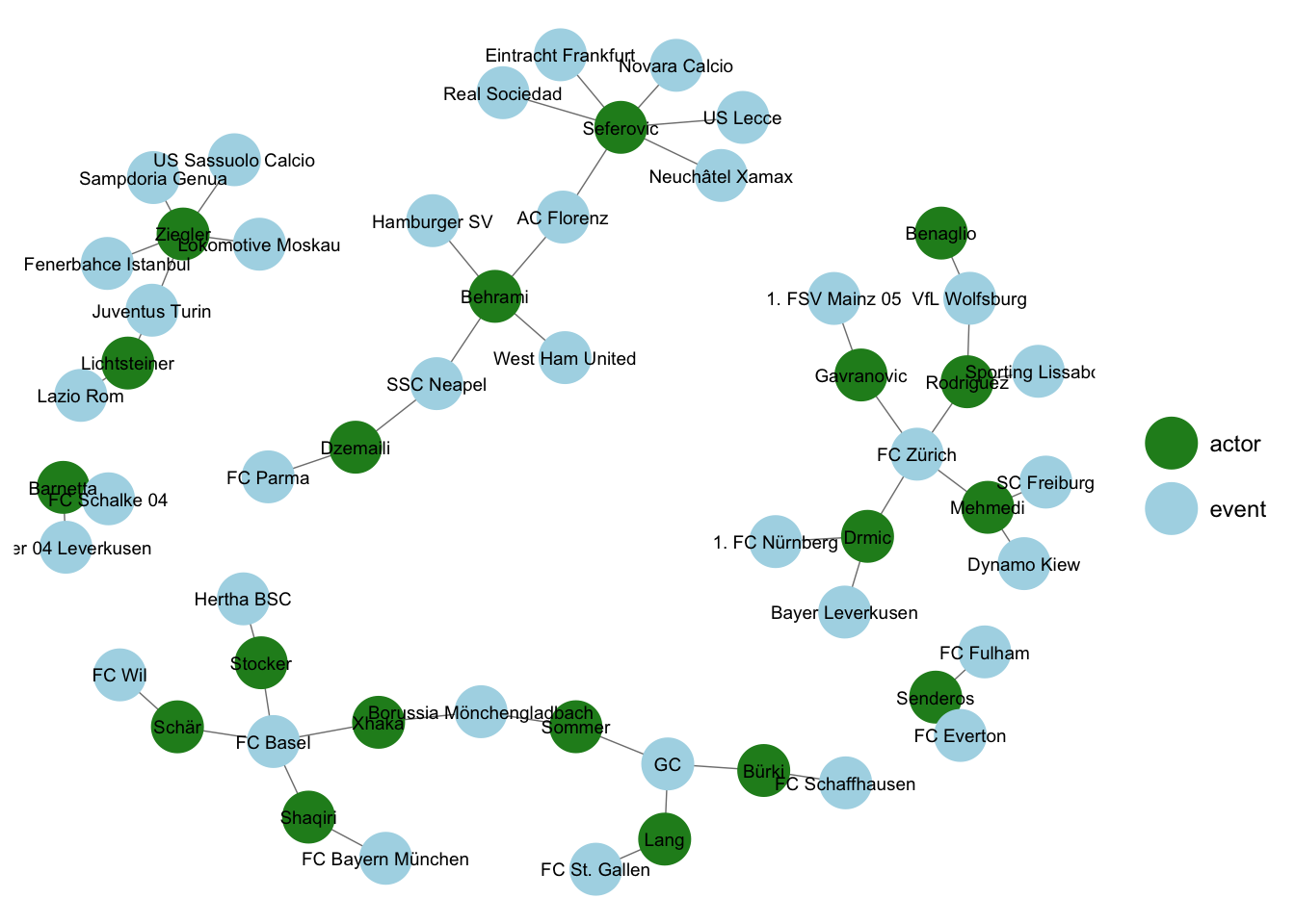
A matrix storing ties for a two-mode network is rectangular and commonly referred to as an incidence or occurence matrix.
##            FC Zürich GC FC Schaffhausen 1. FSV Mainz 05 FC St. Gallen
## Gavranovic         1  0               0               1             0
## Lang               0  1               0               0             1
## Bürki              0  1               1               0             0
## Schär              0  0               0               0             0
##            FC Wil FC Basel
## Gavranovic      0        0
## Lang            0        0
## Bürki           0        0
## Schär           1        1
A projection onto a one-mode network can be achieved by multiplying the rectangular matrix by its transpose. Now players are connected based on whether they played together in the same clubs.
one_mode_projection <- bip_mat %*% t(bip_mat)
diag(one_mode_projection) <- 0 #exclude self-ties
one_mode_projection[1:10,1:10] #look at the first 10 players
## Gavranovic Lang Bürki Schär Sommer Stocker Shaqiri Benaglio
## Gavranovic 0 0 0 0 0 0 0 0
## Lang 0 0 1 0 1 0 0 0
## Bürki 0 1 0 0 1 0 0 0
## Schär 0 0 0 0 0 1 1 0
## Sommer 0 1 1 0 0 0 0 0
## Stocker 0 0 0 1 0 0 1 0
## Shaqiri 0 0 0 1 0 1 0 0
## Benaglio 0 0 0 0 0 0 0 0
## Xhaka 0 0 0 1 1 1 1 0
## Lichtsteiner 0 0 0 0 0 0 0 0
## Xhaka Lichtsteiner
## Gavranovic 0 0
## Lang 0 0
## Bürki 0 0
## Schär 1 0
## Sommer 1 0
## Stocker 1 0
## Shaqiri 1 0
## Benaglio 0 0
## Xhaka 0 0
## Lichtsteiner 0 0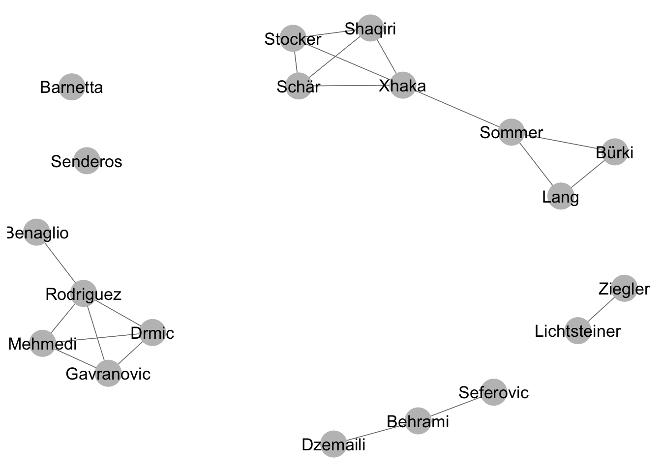
3.4 Network visualization
3.4.1 A word of warning
Network visualizations are at the same time pretty and dangerous. Be aware that nodes will always be placed on a canvas through an algorithm. The choice of a different algorithm can lead to a vastly different illustration. It is thus easy to convey substantive results that are just artefacts of the visualization procedure, for example regarding the centrality of actors. It is in your responsibility to use visualization to augment, not distort interpretation. If you read a network study engaging in “visual interpretation” - look for the numbers. Do they back up the story?
3.4.2 Resources for visualization
For pretty graphs in R, ggnet2 is hard to beat. https://briatte.github.io/ggnet/
For more advanced (and even prettier) visualizations, Gephi is a dedicated open source project (although somewhat buggy). https://gephi.org/
A third, java-based visualization tool is Visone. It is hard to beat when you want to look at different clusters in your network (but contains almost all other network visualization tools as well). https://visone.info
3.4.3 A brief overview over ggnet2()
The command ggnet2() can work with either the adjacency matrix and the attributes-data frame or with the network object.
ggnet2(friends_adjmat,
       label = TRUE,                     # should nodes be labeled?
       arrow.size = 4, arrow.gap = 0.04, # set arrowheads
       node.color = att$Position,        # specify node colors
       palette = 'Spectral')             # use a pretty color-palette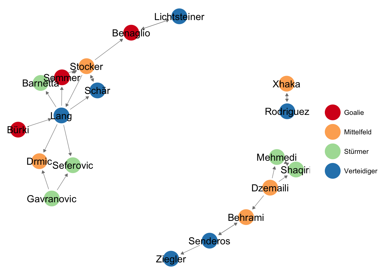
Since all ggnet()-plots are ggplots you can add theme options that you usually use in ggplots:
ggnet2(friends_adjmat,
       label = TRUE,
       arrow.size = 4, arrow.gap = 0.04,
       node.color = att$Position,
       palette = 'Spectral') +
  theme(legend.position = 'bottom') +
  ggtitle("Friendship network of the Swiss national soccer team")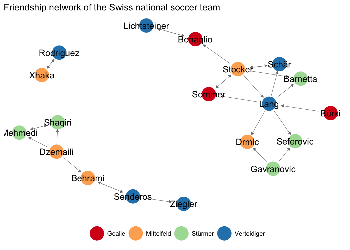
Plus you can save the plots using ggsave():
ggsave(file = 'figures/nw_soccerCH.pdf', width = 15, height = 12, units = 'cm')